Wholesale day-ahead Germany optimization tutorial#
In this tutorial, we will demonstrate how to use the DEBatteryOptimizer to optimize marketing for and operation of a grid-scale battery energy storage system (BESS) in the
German wholesale day-ahead electricity market. We will cover the necessary steps to set up the optimizer, define the parameters, and run the optimization process.
Let us first define the physical parameters of the asset and its grid connection. The parameters we can provide are defined in BatteryParameters:
In [1]: from battery_optimizer.request import BatteryParameters

In [2]: pprint(list(BatteryParameters.model_fields.keys()))
['min_soe',
 'max_soe',
 'min_soe_kwh',
 'max_soe_kwh',
 'charging_efficiency',
 'discharging_efficiency',
 'max_charging_power_kw',
 'max_discharging_power_kw',
 'capacity_kwh',
 'capacity_nominal_kwh',
 'max_daily_cycle',
 'daily_cycle_limit_applies',
 'daily_cycle_limit_penalty',
 'grid_connection_export_kw',
 'grid_connection_import_kw',
 'ramp_rates']
Let us focus on the parameters that we need to define and let the optimizer handle the rest with default values. Here, we will model a standard 1 MW / 2 MWh with sensible efficiencies, (for now) a daily cycle limit of one, and grid connection limits:
In [3]: battery_parameters = {
   ...:     'capacity_kwh': 2000,
   ...:     'min_soe': 0.,
   ...:     'max_soe': 1.,
   ...:     'max_charging_power_kw': 1000,
   ...:     'max_discharging_power_kw': 1000,
   ...:     'discharging_efficiency': 0.95,
   ...:     'charging_efficiency': 0.95,
   ...:     'max_daily_cycle': 1,  # note: just one cycle for now!
   ...:     'grid_connection_export_kw': 1000,
   ...:     'grid_connection_import_kw': 1000,
   ...: }
   ...:
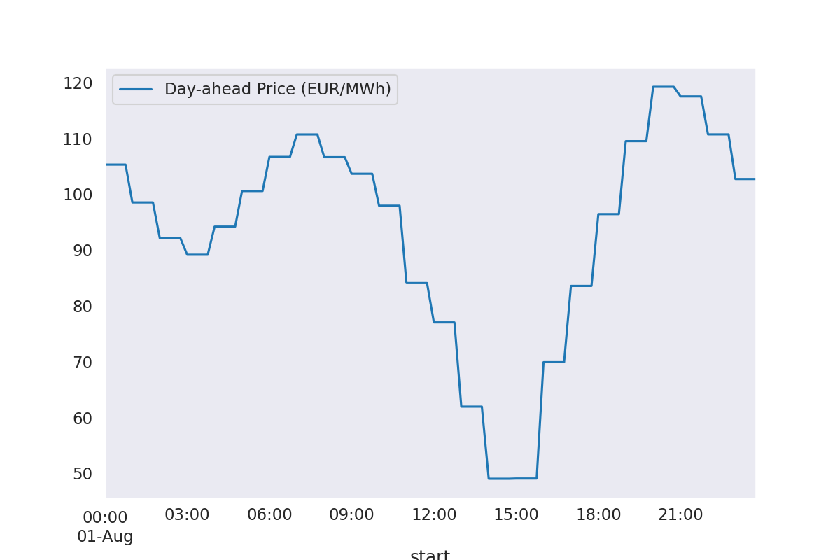
Next we will need a price forecast for the optimization horizon. In lieu of using an actual forecast, we will use realized prices from the EPEX SPOT day-ahead market for Germany. So head over to e.g. the ENTSOE-E Transparency Platform to download historical day-ahead prices for Germany. Here, we did so for August 1, 2025:
In [4]: price_forecast = pd.read_csv(directory / 'data' / 'de_da_prices_2025_08_01.csv', parse_dates=['start'], index_col='start')

In [5]: price_forecast.plot(figsize=(12, 8));

In [6]: plt.show()
We also need to define what the state of energy (SoE) of the battery is at the start of the optimization horizon. Let us suppose the battery starts at 0 MWh stored energy:
In [7]: battery_initial_conditions = {
   ...:     'initial_soe': 0.,
   ...: }
   ...:
There are a lot more parameters we can define to customize the optimization problem to our needs, however for now we keep it simple and just set up the optimizer with the parameters we defined so far.
In [8]: from battery_optimizer.de.battery_optimization import DEBatteryOptimizer

In [9]: problem = DEBatteryOptimizer(
   ...:     request_id='tutorial_de_da_2025_08_01',
   ...:     country='de',
   ...:     user_id='tutorial_user',
   ...:     request_creation_time=pd.Timestamp.now(),
   ...:     asset={
   ...:         'battery_parameters': battery_parameters,
   ...:         'battery_initial_conditions': battery_initial_conditions,
   ...:         'price_forecast': price_forecast.reset_index().to_dict('records'),
   ...:         'battery_marketed': pd.DataFrame(
   ...:             {
   ...:                 'start': price_forecast.index, 'fcr_kw': 0.,
   ...:                 'afrr_capacity_pos_kw': 0., 'afrr_capacity_neg_kw': 0.,
   ...:                 'afrr_energy_pos_kw': 0., 'afrr_energy_neg_kw': 0.,
   ...:                 'bought_intraday_kw': 0., 'sold_intraday_kw': 0.,
   ...:                 'bought_epexIDA1_kw': 0., 'sold_epexIDA1_kw': 0.,
   ...:                 'bought_epexDA_kw': 0., 'sold_epexDA_kw': 0.,
   ...:             }
   ...:         ),
   ...:         'battery_availabilities': pd.DataFrame(
   ...:             {'start': price_forecast.index, 'availability': True}
   ...:         ),
   ...:         'strategy_optimization': {
   ...:             'frequency_min': '15min',
   ...:             'horizon': {'start': price_forecast.index[0], 'end': price_forecast.index[-1]},
   ...:             'markets': ['epexDA'],
   ...:         },
   ...:     },
   ...: )
   ...:

In [10]: problem.solve_optimization_problem()

In [11]: from battery_optimizer.de.result import DEResult

In [12]: result = DEResult.create_dataframe_from_solved_problem(problem)

In [13]: fig, (price_axis, power_axis) = plt.subplots(2, 1, figsize=(12, 8), sharex=True, gridspec_kw={'height_ratios': [1, 3]});

In [14]: fig.subplots_adjust(hspace=0.05);

In [15]: price_axis.plot(price_forecast.index, price_forecast['epexDA'], label='EPEX DA Price / EUR/MWh', color='tab:grey');

In [16]: price_axis.set_ylabel('Price (EUR/MWh)', fontsize='small');

In [17]: power_axis.bar(result.index, result['epexDA_volume_sold_MW'], width=0.01, label='Day-ahead wholesale / MW', color='tab:blue', alpha=0.6);

In [18]: power_axis.bar(result.index, -result['epexDA_volume_bought_MW'], width=0.01, label='Day-ahead wholesale / MW', color='tab:blue', alpha=0.6);

In [19]: power_axis.axhline(0, color='black', linewidth=1.5, linestyle='--');

In [20]: power_axis.set_ylabel('Power (MW)', fontsize='small');

In [21]: energy_axis = power_axis.twinx();

In [22]: energy_axis.plot(result.index, result['soe_target_kwh'].shift(1).fillna(0.) / 1000., label='State of Charge / MWh', color='tab:red');

In [23]: energy_axis.set_ylabel('State of Charge (MWh)', fontsize='small');

In [24]: fig.autofmt_xdate();

In [25]: plt.tight_layout();

In [26]: plt.show();
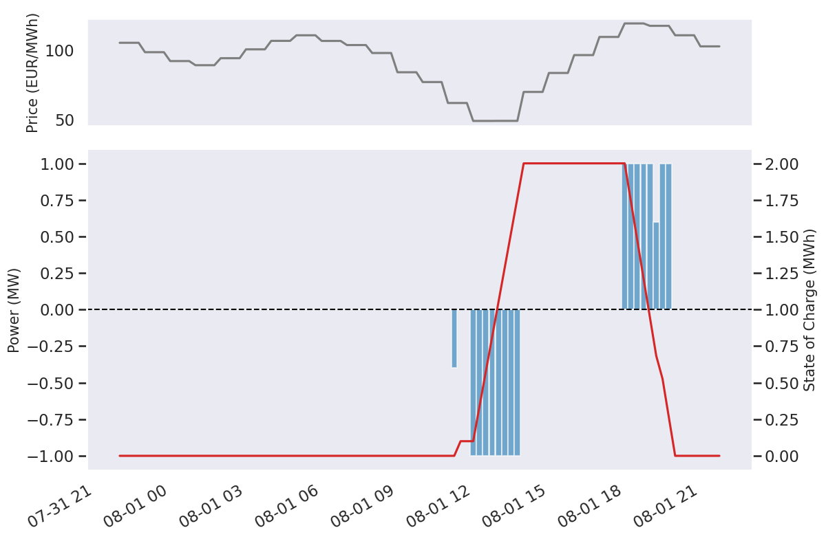
Here we see in blue bars day-ahead market purchases (downwards) and sales (upwards) as proposed by the optimizer. The resulting state of energy (SoE) of the battery is shown in red.
We can see that the optimizer has chosen to fully charge the battery during the low-price period around midday and discharge it during the high-price period in the evening. Note that the price curve for August 1, 2025 exhibits two peaks and the optimizer makes optimal use of this complex price pattern within the constraints we have defined.
In particular, we allowed the optimizer only a single discharge cycle as per the above battery parameters. Let us change that and allow for two full cycles per day and see how the optimization result changes:
In [27]: battery_parameters = {
   ....:     'capacity_kwh': 2000,
   ....:     'min_soe': 0.,
   ....:     'max_soe': 1.,
   ....:     'max_charging_power_kw': 1000,
   ....:     'max_discharging_power_kw': 1000,
   ....:     'discharging_efficiency': 0.95,
   ....:     'charging_efficiency': 0.95,
   ....:     'max_daily_cycle': 2,
   ....:     'grid_connection_export_kw': 1000,
   ....:     'grid_connection_import_kw': 1000,
   ....: }
   ....:
In [28]: from battery_optimizer.de.battery_optimization import DEBatteryOptimizer

In [29]: problem = DEBatteryOptimizer(
   ....:     request_id='tutorial_de_da_2025_08_01',
   ....:     country='de',
   ....:     user_id='tutorial_user',
   ....:     request_creation_time=pd.Timestamp.now(),
   ....:     asset={
   ....:         'battery_parameters': battery_parameters,
   ....:         'battery_initial_conditions': battery_initial_conditions,
   ....:         'price_forecast': price_forecast.reset_index().to_dict('records'),
   ....:         'battery_marketed': pd.DataFrame(
   ....:             {
   ....:                 'start': price_forecast.index, 'fcr_kw': 0.,
   ....:                 'afrr_capacity_pos_kw': 0., 'afrr_capacity_neg_kw': 0.,
   ....:                 'afrr_energy_pos_kw': 0., 'afrr_energy_neg_kw': 0.,
   ....:                 'bought_intraday_kw': 0., 'sold_intraday_kw': 0.,
   ....:                 'bought_epexIDA1_kw': 0., 'sold_epexIDA1_kw': 0.,
   ....:                 'bought_epexDA_kw': 0., 'sold_epexDA_kw': 0.,
   ....:             }
   ....:         ),
   ....:         'battery_availabilities': pd.DataFrame(
   ....:             {'start': price_forecast.index, 'availability': True}
   ....:         ),
   ....:         'strategy_optimization': {
   ....:             'frequency_min': '15min',
   ....:             'horizon': {'start': price_forecast.index[0], 'end': price_forecast.index[-1]},
   ....:             'markets': ['epexDA'],
   ....:         },
   ....:     },
   ....: )
   ....:

In [30]: problem.solve_optimization_problem()

In [31]: from battery_optimizer.de.result import DEResult

In [32]: result = DEResult.create_dataframe_from_solved_problem(problem)

In [33]: fig, (price_axis, power_axis) = plt.subplots(2, 1, figsize=(12, 8), sharex=True, gridspec_kw={'height_ratios': [1, 3]});

In [34]: fig.subplots_adjust(hspace=0.05);

In [35]: price_axis.plot(price_forecast.index, price_forecast['epexDA'], label='EPEX DA Price / EUR/MWh', color='tab:grey');

In [36]: price_axis.set_ylabel('Price (EUR/MWh)', fontsize='small');

In [37]: power_axis.bar(result.index, result['epexDA_volume_sold_MW'], width=0.01, label='Day-ahead wholesale / MW', color='tab:blue', alpha=0.6);

In [38]: power_axis.bar(result.index, -result['epexDA_volume_bought_MW'], width=0.01, label='Day-ahead wholesale / MW', color='tab:blue', alpha=0.6);

In [39]: power_axis.axhline(0, color='black', linewidth=1.5, linestyle='--');

In [40]: power_axis.set_ylabel('Power (MW)', fontsize='small');

In [41]: energy_axis = power_axis.twinx();

In [42]: energy_axis.plot(result.index, result['soe_target_kwh'].shift(1).fillna(0.) / 1000., label='State of Charge / MWh', color='tab:red');

In [43]: energy_axis.set_ylabel('State of Charge (MWh)', fontsize='small');

In [44]: fig.autofmt_xdate();

In [45]: plt.tight_layout();

In [46]: plt.show();
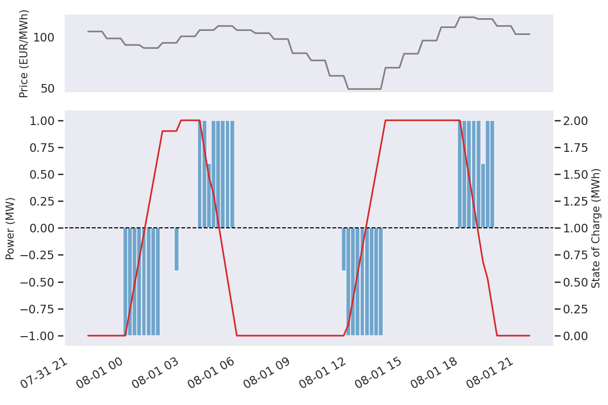
As we can see, allowing for two full cycles per day enables the optimizer to take advantage of the multiple price peaks during the day, resulting in increased revenue from the battery operation.
This demonstrates the flexibility and effectiveness of the battery_optimizer.de.battery_optimization.DEBatteryOptimizer in optimizing battery operations in the German wholesale day-ahead electricity market.